From pressure recordings to a velocity profile.
Turning two sets of laboratory measurements into comparable, dimensionless plots.

A folder full of measurements
The laboratory work began with short pressure recordings at different probe heights. I needed a representative value for each recording, the correct height for each value, and a way to keep two different tests straight.
The details change the picture
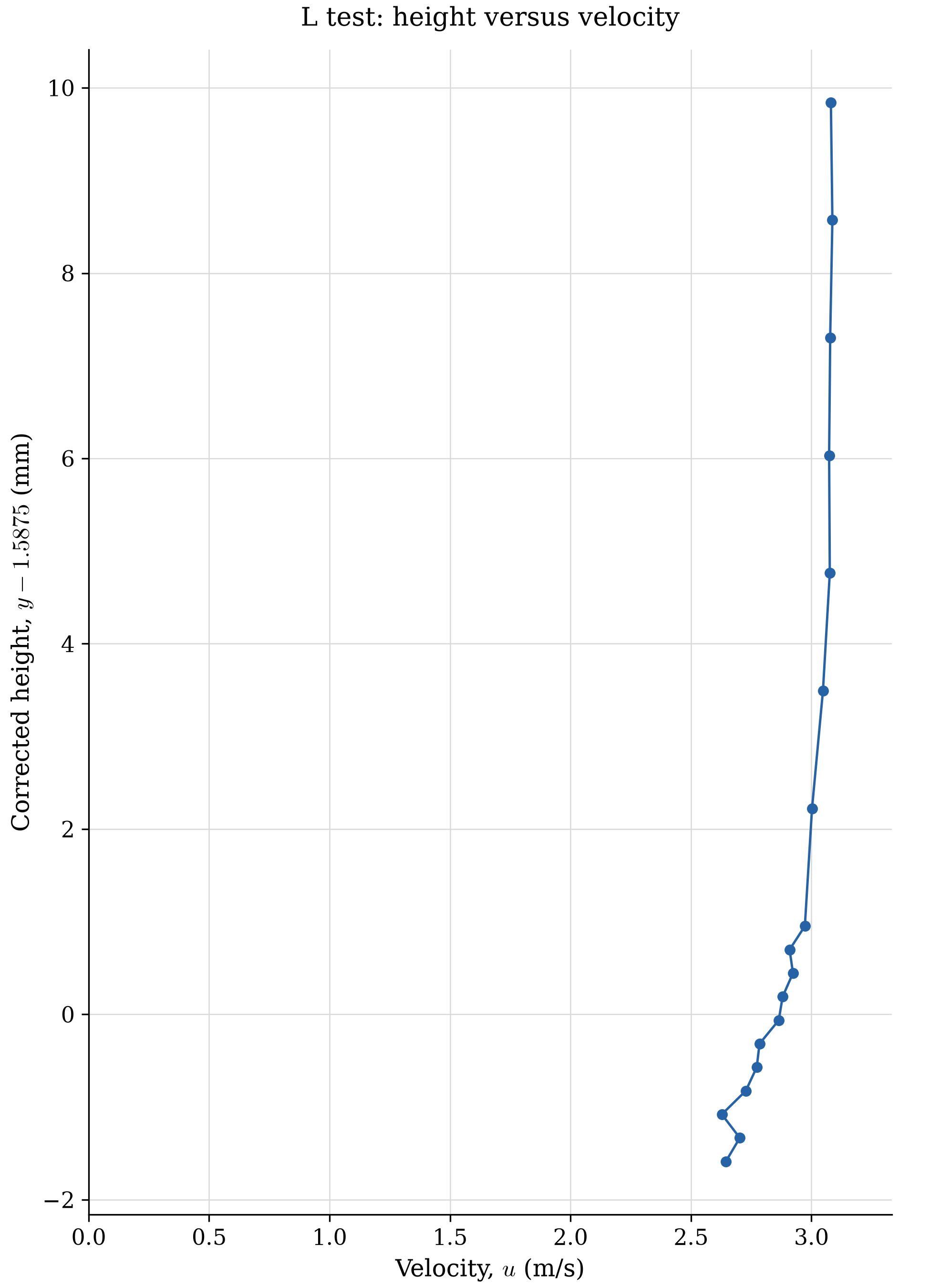
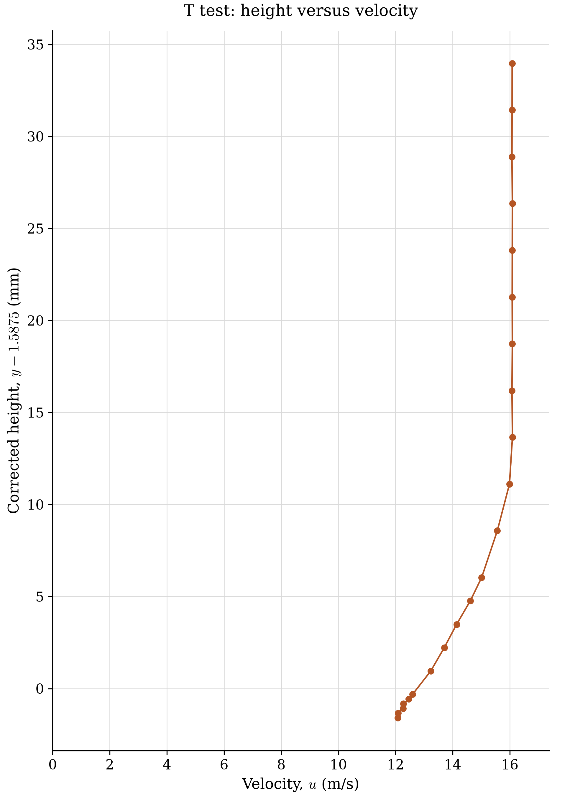
The analysis uses a confirmed 1.5875 mm height correction. It moves from pressure data to velocity profiles, then compares the tests using velocity and height ratios. Boundary-layer thickness was estimated by interpolation at u/U = 0.99.
The result I can point to
The plots above came out of that workflow, alongside a combined workbook. This is the part of experimental work I want to show: the path from recordings to a readable comparison, with units and assumptions kept visible.